12 Steps to Navier-Stokes
Background
Back in my senior year of college I decided to take an Intro to CFD class with the goal of learning more about the theory behind the commercial software I was using to build my FSAE Vehicle Aerodynamics simulations. The final project entailed writing a simulation of Lid-driven cavity flow from scratch in MATLAB. I learned much about programming and fluid dynamics in the process and it’s been a project I’ve wanted to revisit and expand upon ever since.

Sadly, after graduation I lost my Matlab license and with it the chance to fulfill my goal of expanding upon the code I wrote for that project. However times have changed and since I’ve graduated I have become much more familiar with Python and its ecosystem of libraries and packages, In fact, I feel more confident programming in Python than I ever was using MATLAB. CFD became the focus of another one of my projects and I felt that it was the right time to revisit this project as a review and with the aim of re-building the simulation I made in college using Python.
While looking into what building such a simulation would take in Python I stumbled upon Prof. Lorena Barba’s fantastic interactive module 12 Steps to Navier-Stokes. In this module Prof. Barba incrementally builds the code necessary to run a Lid-driven cavity flow simulation from scratch using Jupyter Notebooks to illustrate the process. It fit the goals for this project so well — and also offered a much needed a refresher on the theory — that I decided to embark upon the task of following this module and use this as a chance to write a bit about the experience.
Lessons
The course structure is outlined in the project’s github page which you can take a look at here. It begins by covering the process of discretizing and coding partial differential equations in 1D, then moves to 2D and finally applies the same process to the Navier Stokes equations in 2D.
Even though I had previous experience both in coding with Python and in the theory behind CFD I still found this module extremely useful as a refresher on the topic and as a way to solidify my understanding. Richard Feynman put it best when he said “What I cannot create, I do not understand” and this course succesfully flips this concept on its head by achieving understanding through the process of building the simulations. This is the learning process that has worked for me in the past and it was no difference here.
However, I felt that the modules would be improved upon in some cases if there was a way to see the time-dependant simulations as they evolve in time instead of just plotting initial and final conditions. So, as a way to put my own spin on the project I challenged myself to do just that and I also went ahead and animated all of the simulations. The process was definitely a learning experience but I survived thanks to matplotlib’s great documentation. I am excited to share with you some of my personal favorites from the course below. If you want to take a more in depth look at how I made these or if you’re the kind that prefer’s code over words, do not despair! You can check out my github repo [here].
1D Simulations
1D Diffusion
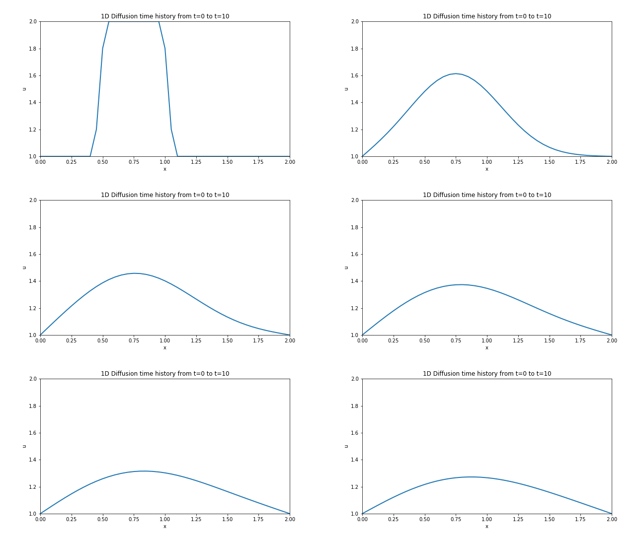
Although this was the third step in the project, I believe it was the first one that yielded a worthy animation. The process of diffusion is ubiquitous and can be seen in pretty much any process that has a gradient in it’s quantity applied over a length. So it was very satisfying to see that common phenomena simulated and animated directly on my screen.
You can follow this link to the Jupyter Notebook [Step 3] where I outlined the process I followed to obtain this plot along with the relevant code and equations involved in the discretization.
1D Burgers Equation
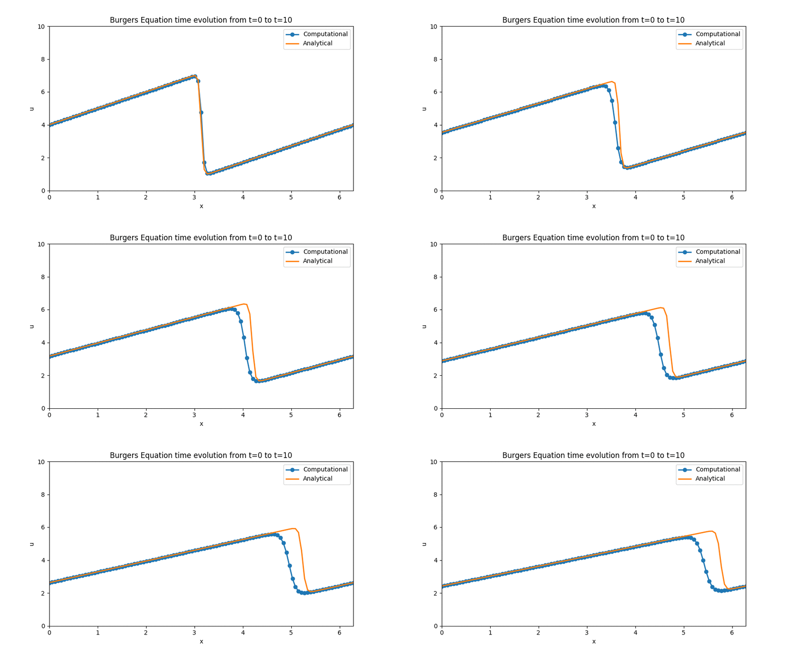
The interesting part about this simulation is that the equation we modeled has a well known set of analytical solutions that we can use to analize the performance of our numerical discretization scheme. It also made use of periodic boundary conditions — something I hadn’t even heard of before — which added an interesting learning challenge to this step. There was also a very brief detour on the use of Sympy to perform analytical derivatives that was brand new territory for me, but which I am now sure will come in handy in the future.
Again, you can follow this link to the Jupyter Notebook [Step 4] where I outlined the process I followed to obtain this plot along with the relevant code and equations involved in the discretization.
2D Simulations
2D Diffusion
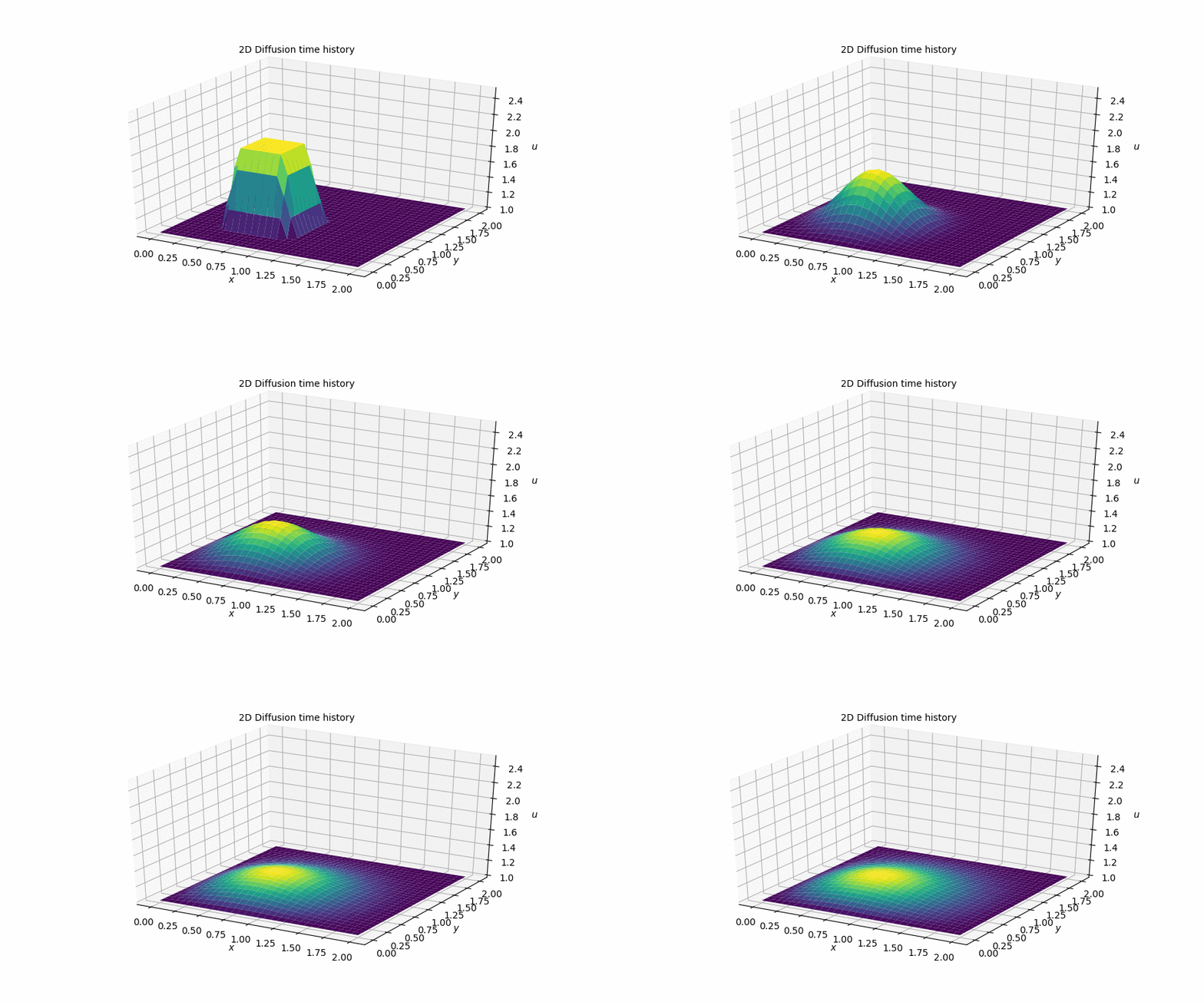
This simulation is the direct analogue of the 1D Diffusion simulation that I showed above. That is, it attempts to model the exact same behaviour but in two dimensions. What I found most noteworthy about this step was the introduction of vectorized notation to speed-up the iterative process. The performance gains were incredible! My code went from taking over 3s to perform a simulation to 0.05s. It was definitely a bit humbling to reallize how much more I have yet to learn about how to write good Python code.
Similarly, You can follow this link to the Jupyter Notebook [Step 7] where I outlined the process I followed to obtain this plot along with the relevant code and equations involved in the discretization.
2D Poisson
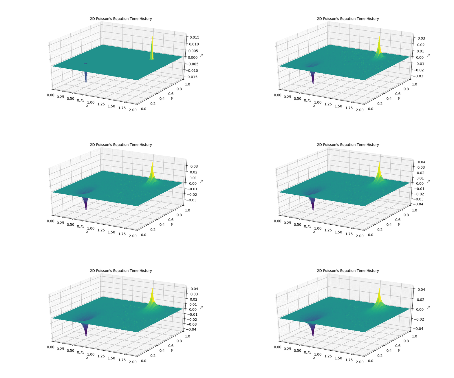
The poisson equation is an interesting stepping stone in this project because it can be understood as the solution a problem that is found in the full Incompressibl Navier-Stokes equations: the lack of a coupling between pressure and velocity. However, Poisson’s equation is not time dependent and therefore the plot above only represents the first couple of timesteps that the simulation took on its way to its steady state.
If you’d like to, you can follow this link to the Jupyter Notebook [Step 10] where I outlined the process I followed to obtain this plot along with the relevant code and equations involved in the discretization.
Cavity-Flow Simulation
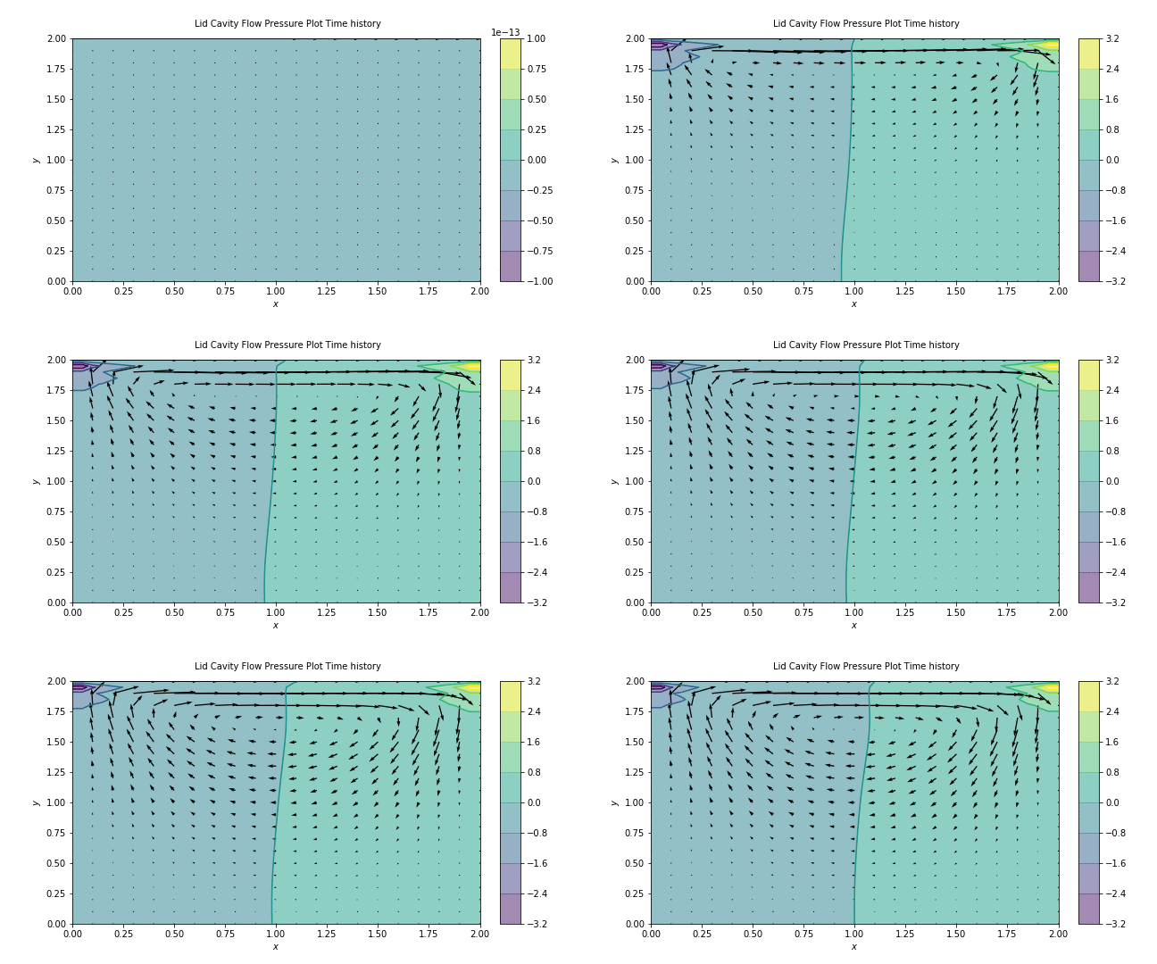
And here we have it: The lid driven cavity flow simulation that I worked on in college re-built in Python as the crowning achievement of the 12 Steps to Navier Stokes! As you would expect, it shows a spiral pattern and two distinct pressure zones. Sadly because this took forever to run on my machine, this animation only shows a quarter of a second so the flow pattern shown here is not fully defined. However, I am very happy with the results and the overall presentation. I think that adding animations really improved the quality of the final project since it helped me gain more of an intuition about the phenomena and how it evolved over time. Now that I have reached the same point I was at when I finished my Intro to CFD course I can start expanding upon this code in more exciting directions and create more interesting and complex simulations. It’s only the beginning!
Last but not least, you can follow this link to the Jupyter Notebook [Step 11] where I outlined the process I followed to obtain this plot along with the relevant code and equations involved in the discretization.
Conclusion & Next Steps
I would wholeheartedly recommend this interactive course to anyone who has any interest in CFD or wants to practice more Python. I personally got out of this experience a bunch of new skills: making animations in python, how to vectorize code for faster computations, sympy for doing symbolic manipulation and, of course, how to build simple CFD simulations in Python.
Yet, now that I have caught up to my previous CFD knowledge I am really curious as to what it would take to modify this code to solve for an arbitray 3D geometry. The goal would be to see if I can feed it a CAD assembly — probably as a STEP file — and get it to identify the geometry and simulate the flow over it in Python.
I know I am getting a bit ahead of myself here since I still feel I have a lot more to learn about CFD before I ever get to write my own solver. So, I’ve decided that before I delve into writing code I want to investigate the current landscape of Open Source CFD programs and get more familiar with the options out there such as OpenFOAM. Perhaps as a Future project, maybe??
Hopefully in a couple of weeks time here is where I link you to it!
If you’re also interested in projects that live at the intersection of Computer Science and Aerospace, let’s talk! I have many contact links on my about page and I would love to hear your thoughts.